CS 548 - Robot Motion Control and Planning
Assignment #2: Potential Field Methods
Ali Nail İNAL
Bilkent University,Electrical&Electronics Engineering Department
Instructor: Asst. Prof. Uluç SARANLI
Introduction
As a assignment for the robot motion and control course, we will examine the potential field methods as a part of the path planning algorithms. Potential field methods, compared to bug algorithm used in first assignment, provides us many advantages, especially about dimension of the configuration spaces (we are no more bounded to 2D spaces). It can be applied to spaces that are bounded by sphere boundary and all the obstacles are spheres, also, its application can be expanded to star-spaces(spaces that can be obtained by diffiomorphism from sphere-spaces) and Non-Euclidian spaces. These methods have the information on obstacle, boundary and goal positions, thus in order to apply this method you need a global map.
Potential Field methods use potential function U: ![]() ,
which is differentiable and real valued and can be viewed as energy, in order
to navigate on the calculated minimum potential. Gradient of the U,
,
which is differentiable and real valued and can be viewed as energy, in order
to navigate on the calculated minimum potential. Gradient of the U, ![]() points in the direction that locally maximally
increases U. Using gradient we can obtain a vector field that assigns the
maximum U direction for every point on a manifold. Since we think U as energy
then, gradient can be intuitively viewed as forces acting on a positive charge
particle robot [1]. If we think obstacles as also positive charged and goal
point as a negative charged particle, it will give the basic idea of
potentials. Since particle will be attracted to goal point and repelled away
from obstacle, path will be through the minimum potential.
points in the direction that locally maximally
increases U. Using gradient we can obtain a vector field that assigns the
maximum U direction for every point on a manifold. Since we think U as energy
then, gradient can be intuitively viewed as forces acting on a positive charge
particle robot [1]. If we think obstacles as also positive charged and goal
point as a negative charged particle, it will give the basic idea of
potentials. Since particle will be attracted to goal point and repelled away
from obstacle, path will be through the minimum potential.
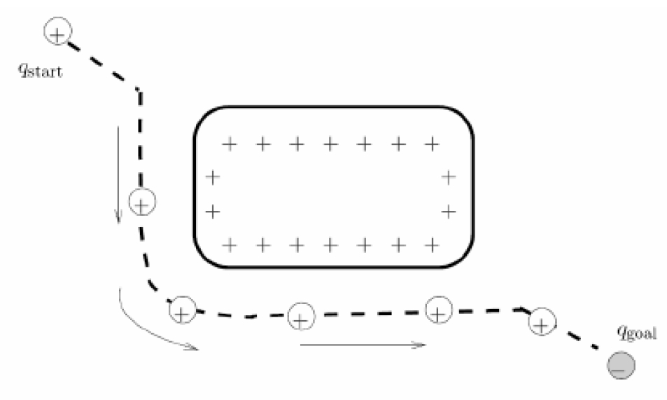
Figure 1 - Potential Field from the electrical charges idea.
In this assignment, we hope to implement two different potential function to observe their performances, and compare them in several aspects. One of them is attractive-repulsive potential functions that have the same idea mentioned above with different functions, and navigation function is a complete and improved version of the first one. They will be examined further in algorithms section.
Problem
Description
As it is mentioned introduction, our main objective
is to implementation of the attractive-repulsive potential function and
navigation function as path planners using gradient-decent algorithm. A point
robot will be moving from the start point to goal point in the 2D sphere world
(boundary is a 2D sphere and all obstacles are sphere). Requirements stated in
the assignment are;
i.
Implement a configurable simulation
platform for 2D sphere world, where number of obstacles, their radius and
positions can be chosen with ease.
ii.
Implement a planner that uses
gradient-decent algorithm with attractive-repulsive potential functions, where
planner has access to global map.
iii.
Implement a planner with navigation
function in the simulation platform.
iv. Compare the two implementation with respect to their performance, speed of convergence, difficulty of implementation or relevant issues, using a number of different example settings for both of them.
Algorithm
For this project,
we implemented two potential functions in gradient descent algorithm, in order
to robot to move towards goal point it moves at every step (or every
infinitesimal time interval) proportional with -![]() .
It is the velocity component that we use in gradient descent for preparing next
step as in the
.
It is the velocity component that we use in gradient descent for preparing next
step as in the ![]() formula.
formula. ![]() is the step size for the ith
iteration, however, we take it as constant for the whole algorithm. Short
description of the gradient decent algorithm is;
is the step size for the ith
iteration, however, we take it as constant for the whole algorithm. Short
description of the gradient decent algorithm is;
While ![]()
1.![]()
2. i=i+1;
End
Short descriptions of the potential functions are given in the next chapters.
→Attractive-Repulsive
Potential
For
attractive-repulsive potential, we find both potentials and their gradients and
then by summing them we obtain the potential and gradient acting on the point.
The attractive
potential is the potential acting on the robot with respect to the goal point,
gradient of which has the attractive effect towards goal on the robot. It is
proportional with ![]() (distance from goal to current position) and
with threshold
(distance from goal to current position) and
with threshold![]() function changes its behavior in order to
balance the magnitude of the potential. Around the goal point it is preferable
to use the quadratic potential since it is differentiable and makes it easy to
force robot towards goal with big magnitudes, however, quadratic potential
became too large for the far away points, thus for these points (differed by
threshold distance) linear relation to
function changes its behavior in order to
balance the magnitude of the potential. Around the goal point it is preferable
to use the quadratic potential since it is differentiable and makes it easy to
force robot towards goal with big magnitudes, however, quadratic potential
became too large for the far away points, thus for these points (differed by
threshold distance) linear relation to![]() will be enough. Thus attractive potential functions will be;
will be enough. Thus attractive potential functions will be;
Repulsive
function keeps the robot away from the obstacle. Strength of the repulsive
force is related with the distance to the obstacle’s nearest point( ![]() ), and if the robot is far enough to the
obstacle we can use the threshold
), and if the robot is far enough to the
obstacle we can use the threshold ![]() to ignore the repulsive potential. Then, the
potential will be;
to ignore the repulsive potential. Then, the
potential will be;
![]()
And the total
potential and total gradient will be;
![]()
→Navigation
Function
Navigation function
is potential function that guarantees to have a single minimum, and it will be
located at goal position for a sufficiently large K. It considers all obstacles
at every point and potential is always
unitary value at obstacle boundaries and zero value at goal point. Navigation
function is;

![]()
![]() can be thought as the repulsive function and
distance square can be thought as attractive function. Since
can be thought as the repulsive function and
distance square can be thought as attractive function. Since ![]() is used as
sharpening function, as K increases this function will make the slope of
the potential from start through goal will increase and the force on the robot
will be bigger however, if it is too steep around the goal, it will become more
flatter around the start point and it will make the time spent on the path
increase. Gradient of the navigation function is calculated similar to the
first functions;
is used as
sharpening function, as K increases this function will make the slope of
the potential from start through goal will increase and the force on the robot
will be bigger however, if it is too steep around the goal, it will become more
flatter around the start point and it will make the time spent on the path
increase. Gradient of the navigation function is calculated similar to the
first functions;
![]()

![]()
Implementation and Results
Simulation environment is prepared on MATLAB platform such that, all the requirements from the assignment is provided. Gradient descent algorithm implemented and step size chosen about one percent of the boundary width. Potential functions are implemented as told in the algorithm section.
As the first case we choose a simpler case, and simulate it with attractive-repulsive potential functions. Results obtained are shown below;
Figure 2: Simple Attraction-Repulsion Case
For this simple case, it works. As it can be seen from the potential graph, it creates a slope towards the goal point. However, there are still local minima where robot may stick. For example is the robot is perpendicular to the obstacle, and if the center of the obstacle on the line that passes through robots position and goal point, then it will stick at that point, since it is a local minimum. Though, this is not a stable local minima, since if it takes a perturbation from x axis it will continue to goal point.
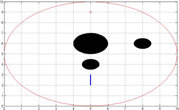
Figure 3: Simple Stuck Case for Attractive-Repulsive Potential
Then, let us simulate a simple navigation function case;
Figure 4: Simple Navigation Function Case
In this case, we use navigation function, with K=3 and it reaches the goal point without a problem. As it can be seen from potential plot and gradient plot, it is always go towards the goal point, no matter where the starting point inside the boundary.
Let us now compare the performance of the both function at a more complicated situation;
First, we use attractive-repulsive potential functions,
Figure 5: Attractive-Repulsive case
Figure 6: Navigation case K=7
As it can be seen, navigation function’s potential more steeper towards goal then the attractive-repulsive case, it also shows in the results as simulation step repetition number, navigation function completes simulation in 2064 unit time when K=7 and 59 unit time when K=5, however, attractive-repulsive function completes simulation in 2439 unit time, thus speed of convergence in navigation function is really higher than the attractive-repulsive case. And if we add some more obstacles to the map, then, attractive-repulsive function cannot obtain the result.
Figure 7: Attractive Repulsive function failed
Since eta chosen larger, attractive-repulsive function cannot reach the goal position. However, navigation function reached there in a very small time interval, since it is a complete method.
However, since step size is limited navigation function can also fails;
Figure 8: Navigation function failed (at left)
If we use step size not small enough, it may fail in some situations, like observed in the figure, however, if we make it smaller speed of convergence will decrease seriously, like in alpha 0.001 cases, although it succeeded the path planning, time spent increase to the 15568 unit time.
One more thing to mention about navigation function would be its relation with K. As it can be seen in the following figure, like low K values, much higher K values also cause trouble, since the start point may stay on the flatter side and speed of convergence would decrease much more than expected.
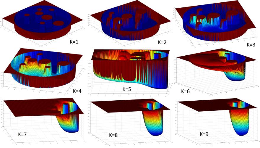
Figure 9: Navigation function potential for different Ks
As it can be observed after K=6, system starts to get more flat on the far side of the goal point. Thus, the time it spends will increase.
Conclusion
Our main goal in this assignment is to implement attractive-repulsive potential function and navigation function in 2D sphere world. In this environment, we compare them and realize that, although attractive-repulsive potential function is easy to implement and gives the short distance path, it does not work in all environments, and its speed of convergence is really low. Additionally, navigation function is a complete method and its speed of convergence is really high, however, it cannot gives the shortest path, and choosing K may also cause problem, if it does not choosen well.
Compared to bug algorithms, potential field methods are better and easy to implement, though it requires more information about environment. If the environment is static, for example a town map, it would work better for the path planning, however, if the dynamic elements are very effective, then it may loose its advantage, if the global map si not updated very frequently.
References
· [1]"Principles of Robot Motion" by Howie Choset etal., MIT Press, 2005, ISBN: 0-262-03327-5.
· [2]"Planning Algorithms" by Steven M. LaValle, Cambridge University Press, 2006, ISBN: 0521862051