![]()
CS 548 - Robot Motion Control and Planning
Assignment #3: Visibility Graph Method
Ali Nail İNAL
Bilkent University,Electrical&Electronics Engineering Department
Instructor: Asst. Prof. Uluç SARANLI
Introduction
For the third homework of the Robot Motion Control and Planning course, we intended to implement one of the deterministic roadmap methods, visibility graph method. Unlikely to the bug algorithms and potential field methods, visibility graphs (and all roadmaps) aims to be general, so that, they can be used for the same environment every time without complex calculations, like a lookup table for the calculators. Also, since you have the stored data to use for the roads, you can find the optimal roads that can be in the roadset.
Additionally, we plan to use a polygonal robot, in this case a triangular robot, since it would be more realistic. However, in order to use a polygonal robot, we need to work on the configuration space, for point robots configuration space and workspace are not different, and for this we will implement star algorithm. Moreover, since the road to be chosen will be more specific, we can use a search algorithm to find the optimal choice. Thus, we will implement A* search algorithm for this project.
Problem
Description
As it is mentioned introduction, our main objective
is to implementation of the visibility graphs method for the polygonal world. A
triangular robot will be moving from the start point to goal point in the 2D
polygonal world (boundary and all obstacles are polygonals). For the sake of
the simplicity, triangular robot will only translate, it will not rotate in any
direction. Requirements stated in the assignment are;
i.
Implement a general algorithm to
construct configuration space obstacles based on the robot’s shape and the
workspace.
ii.
Build visibility graph for the polygonal
configuration space.
iii. Implement search algorithm to obtain an optimal map for random start and goal locations using visibility graph.
Algorithm
For this project,
as mentioned in problem description section, there is 3 main requirements for
implementation. First we will implement star algorithm to obtain the
configuration space. Star algorithm can be used for obtaining R2
configuration space obstacles from its workspace for the convex obstacles. It
is practical to for convex obstacles, however, we need to obtain a
configuration space for all obstacles, thus we decided to use
DelanuayTriangulation method, an algorithm that can divide any concave
polygonal obstacle in to several triangles,that are always convex. Thus after
finding the configuration space obstacles for all triangles we can again put
them in together and obtain the original concave obstacles’ configuration space
representation.
→Star
Algorithm:
This algorithm
specifically used for representing configuration space obstacles in in R2. It checks the edges and the
vertexes of the both robot and the obstacle for the intersections. It defines
two types of contact. Type A contact is the contact between obstacles vertex
and the robot edge, and the type B contact is the contact between robot vertex
and the obstacle edge, if both are edge to edge then it is both considered as
type A and B. If they provide the condition to be one of the types, then the
vertexes of the configuration space obstacle defined by star algorithm. The
position of the obstacle representation will also be correct and there will be
no need to adjust their positions. It uses normals of the edges to control
whether is it paralel to the one edge of the other object. If it is not, it
defines two vertex for the object. Conditions can be obtained from [1].
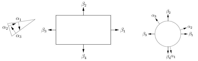
Figure 1: Normals of the obstacles
→Delaunay
Triangulation:
This method tries
to find a set of triangles such that each of the points of a given point set
will be a vertex for the triangles. Additionally, it tries to maximize the
minimum angle of generated triangles. It is very useful to divide concave
obstacles to convex triangles as it is seen in the below:
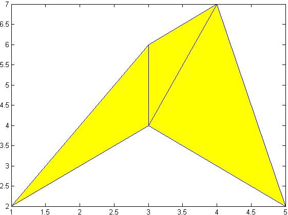
Figure 2: An obstacle divided to triangles using Delaunay Triangulation
→Visibility
Graph:
Visibility graph
method is one of the deterministic roadmap methods and gives us an optimal path
that is defined from the set of visibility graph roads. This method considers
the vertices of the obstacles and the start and goal point as the nodes. Only
on the paths between the nodes can be used. Generally, the linear path is
prefered but also higher order polynomial paths can also defines the paths.
Additionally, it defines cost functions, generally euclidian distance, and use
these to find the optimal path for the given criteria. An example of the
visibility map is given below:
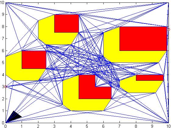
Figure 3: Visibility Graph Example with configuration space obstacles
→A*
Search Algorithm:
A* search algorithm
is a complete best-first graph search algorithm. It gives the optimal solution
from the choice set with given heuristic function (cost function). Its details
can be found in the [1]. In our assignment, we use euclidian distance from nodes
to goal as heuristic function.
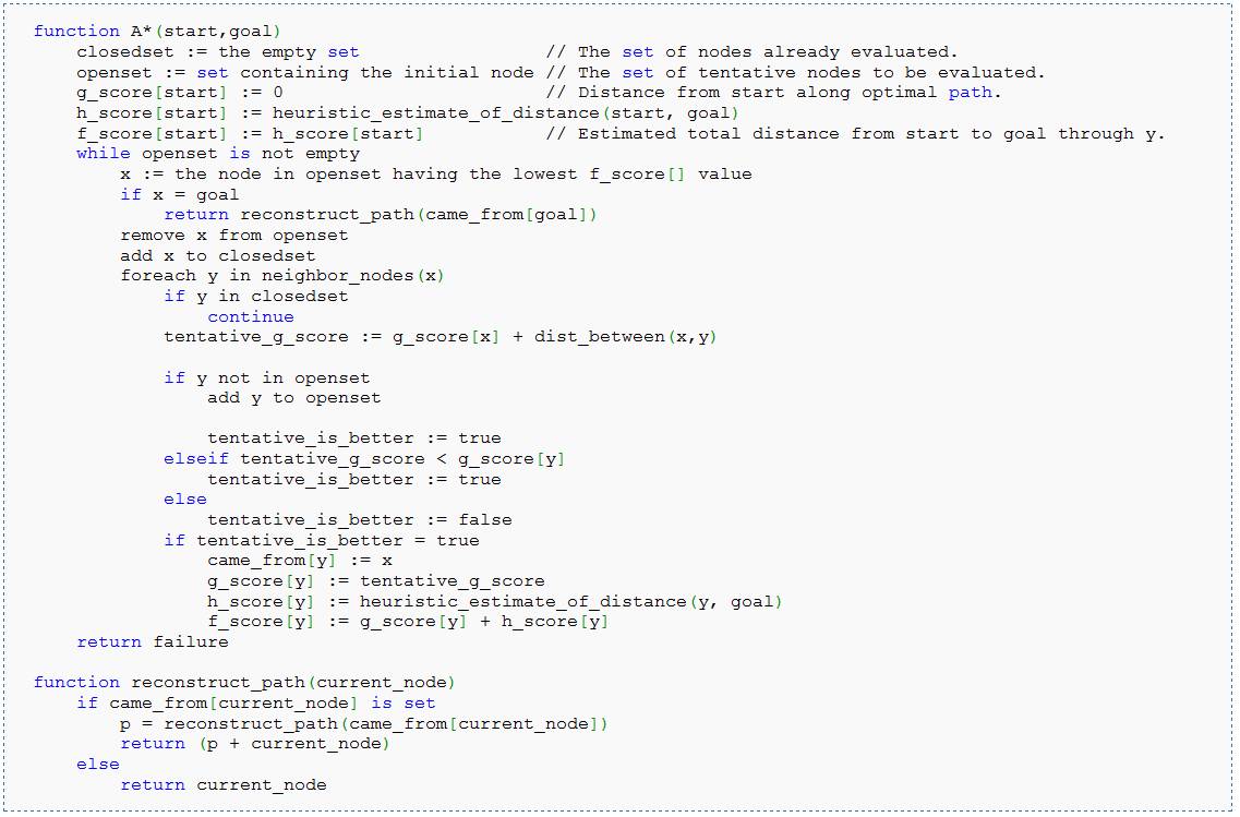
Figure 4: Pseudo-code of the A* algorithm [3]
Implementation and Results
Simulation environment is prepared on MATLAB platform such that, all the requirements from the assignment is provided. In order to obtain configuration space, star algorithm implemented with delaunay triangulation. Since finding whether obstacle is convex or concave is problematic, we apply triangulation to all the obstacles. We obtain the configuration space of the workspace for a triangular robot.
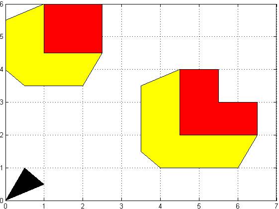
Figure 5: Basic
Configuration space(yellow) with the obstacles(red) and robot(black) shown in
it
By changing orientation and size of the robot we can obtain different configuration spaces:
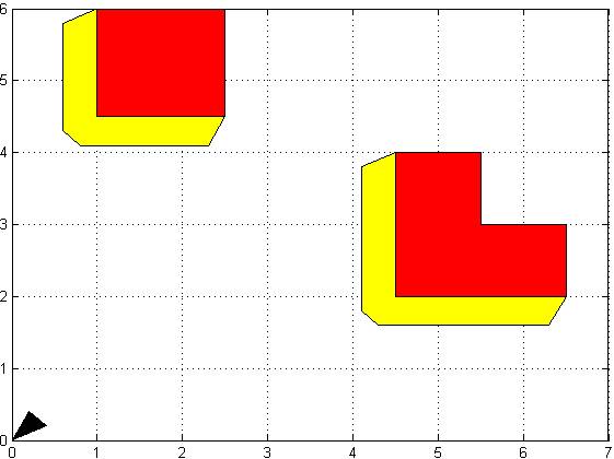
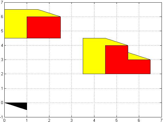
Figure 6: Configuration space for different Obstacles
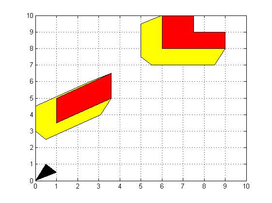
Figure 7:Configuratrion space for different obstacles
Since, the implementation of the star algorithm successful, configuration space obstacles for the visibility graph are ready. Thus, we implement visibility graph as it is described in the book[1].
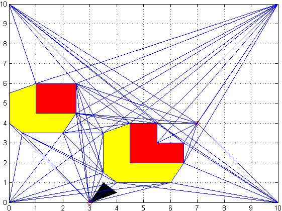
Figure 8: A Basic Visibility Graph example
It can also be reduced by eliminating the unnecessary ones as described in [1]. That way, search algorithms will work more effectively, in shorter times.
Also we can apply these to more complicated environments, like in the following example.
Figure 9: Complicated Visibility Graph example
After we obtain visibility graphs, we use it in for the path plannig using A* algorithm. It worked on all the visibility graphs that I obtained.
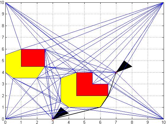
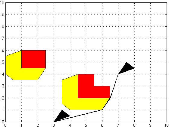
Figure 10: Basic A* solution
It also gives optimal results for the more complex environments.
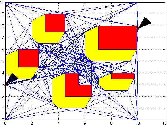
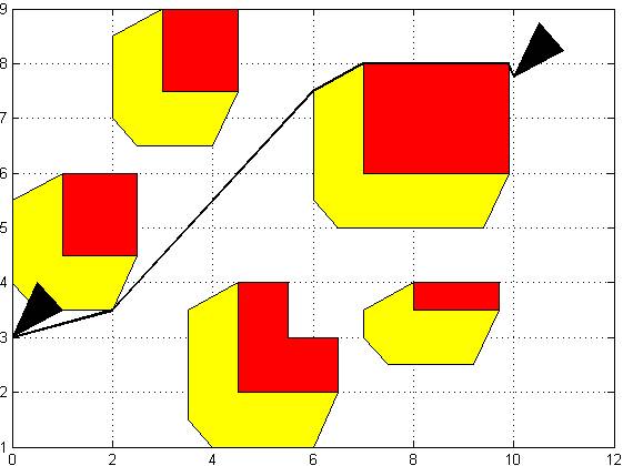
Figure 11: More Complex Environment
However, if the starting point and goal point is not connected then it cannot give a solution:
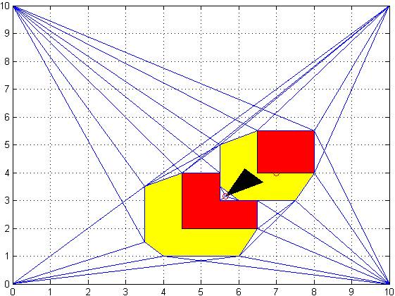
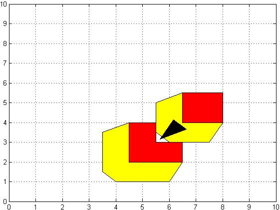
Figure 12: No solution Starting point is blocked
Conclusion
Our main goal in this assignment is to implement visibilty graphs method to polygonal environment with a non-point robot in order to make deterministic roadmap planing. Although it is a complete method, access to global map is a disadvantage for the method. Main advantage of the algorithm is the adjustable cost function. By changing cost function, one can choose safe roads, or may prefer one optimal solution to another. Additionally, working on the configuration space would make the planing more reliable and it is not hard for a polygonal modeled environment, and once it is obtained, it can be used for a robot for all possible orientations, since it can be calculated without much effort. In order to develop this simulation environment, it can be generalized for all the polygonal robots.
References
· [1]"Principles of Robot Motion" by Howie Choset etal., MIT Press, 2005, ISBN: 0-262-03327-5.
· [2]"Planning Algorithms" by Steven M. LaValle, Cambridge University Press, 2006, ISBN: 0521862051
[3]A* Search Algorithm,Wikipedia Encyclopidia,taken 31.03.2010